High-dimensional sparse variable selection
This is the complete supplied example, presented as display-only code so building the documentation site does not allocate the 50,000-predictor design matrix or run the MCMC job. Download the original R Markdown source.
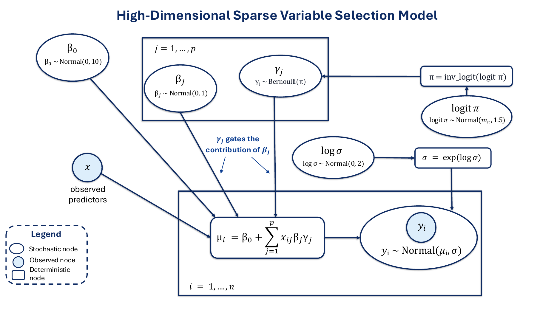
Example: Bayesian variable selection
A sparse Gaussian regression model with binary latent inclusion indicators.
\[ \gamma_j \mid \pi \sim \operatorname{Bernoulli}(\pi), \qquad j = 1,\ldots,p . \]
\[ \beta_j \sim \operatorname{Normal}(0, 1), \qquad \alpha \sim \operatorname{Normal}(0, 10), \qquad \log \sigma \sim \operatorname{Normal}(0, 2). \]
\[ \operatorname{logit}(\pi) \sim \operatorname{Normal}(-4.6, 1.5). \]
\[ \mu_i = \alpha + \sum_{j=1}^p \gamma_j \beta_j x_{ij}, \qquad y_i \mid \alpha, \boldsymbol\beta, \boldsymbol\gamma, \sigma \sim \operatorname{Normal}(\mu_i, \sigma), \qquad i = 1,\ldots,n . \]
The posterior inclusion probability for predictor (j) is
\[ \Pr(\gamma_j = 1 \mid y), \]
and the posterior distribution of the selected regression effect is summarized using
\[ \gamma_j \beta_j. \]
library(hobbs)
library(coda)

set.seed(123)

# -------------------------
# Simulate sparse regression data
# -------------------------

n = 500L
p = 50000L
s = 8L

x = matrix(rnorm(n * p), nrow = n, ncol = p)
x = scale(x)

active = sort(sample.int(p, s))

beta_true = numeric(p)
beta_true[active] = c(2.4, -2.1, 1.8, -1.6, 1.4, -1.2, 1.0, -0.9)

alpha_true = 0.5
sigma_true = 1.0

y = as.numeric(alpha_true + x %*% beta_true + rnorm(n, 0, sigma_true))
y = as.numeric(scale(y, center = TRUE, scale = FALSE))

cat("n:", n, "\n")
cat("p:", p, "\n")
cat("true active predictors:", active, "\n")
cat("true non-zero betas:\n")
print(data.frame(j = active, beta_true = beta_true[active]))

# -------------------------
# Bayesian variable-selection model
# -------------------------
# gamma(j) = 0 excludes predictor j
# gamma(j) = 1 includes predictor j
#
# The likelihood is written in the Kuo-Mallick form:
#   mu_i = alpha + sum_j gamma_j beta_j x_ij

model_src = '
param beta(p) sampler=slice;
param logsigma(1) sampler=slice;
param logit_pi(1) sampler=slice;
dparam gamma(p, 0, 1);

func y_lpdf() {
  double sigma = exp(logsigma(1));

  for (i = 1:n) {
    y(i) ~ dnorm(mu(i), sigma);
  }
}

block beta(j) {
  beta(j) ~ dnorm(0, 1);

  if ((j == 1) || (gamma(j) != 0)) {
    y_lpdf();
  }
} cache mu(n) {
  int nactive = 0;
  int active[p];

  for (k = 2:p) {
    if (gamma(k) != 0) {
      active[nactive] = k;
      nactive += 1;
    }
  }

  for (i = 1:n) {
    mu(i) = beta(1) * x(i,1);

    if (nactive > 0) {
      for (a = 0:(nactive-1)) {
        int kk = active[a];
        mu(i) += beta(kk) * x(i,kk);
      }
    }
  }
} update mu(n) {
  if ((j == 1) || (gamma(j) != 0)) {
      for (i = 1:n) {
        mu(i) += (proposal(beta(j)) - current(beta(j))) * x(i,j);
      }
  }
}

block logsigma(1) {
  logsigma(1) ~ dnorm(0, 2);

  y_lpdf();
}

block gamma(j) {
  double pi = inv_logit(logit_pi(1));
  gamma(j) ~ dbern(pi);

  y_lpdf();
} update mu(n) {
  if (j != 1) {
      for (i = 1:n) {
        mu(i) += (proposal(gamma(j)) - current(gamma(j))) * beta(j) * x(i,j);
      }
  }
}

block logit_pi(1) {
  double pi = inv_logit(logit_pi(1));
  logit_pi(1) ~ dnorm(-4.6, 1.5);

  for (k = 2:p) {
    gamma(k) ~ dbern(pi);
  }
}
'

mod_data = list(
  n = as.integer(n),
  p = as.integer(p),
  y = as.double(y),
  x = x
)

fit = hobbs(
  model = model_src,
  data = mod_data,
  samples = 2000L,
  burnin = 1000L,
  out = "hd_var_selec.bin"
)

draws = read_hobbs("hd_var_selec.bin")

# -------------------------
# Posterior summaries
# -------------------------

# beta[1] is the intercept.
# Predictor j corresponds to beta[j + 1] and gamma[j].
beta_cols = paste0("beta[", seq_len(p), "]")
gamma_cols = paste0("gamma[", seq_len(p), "]")

missing_beta = setdiff(beta_cols, names(draws))
missing_gamma = setdiff(gamma_cols, names(draws))

if (length(missing_beta) > 0L) {
  stop(
    "Missing beta columns, including: ",
    paste(head(missing_beta, 10L), collapse = ", ")
  )
}

if (length(missing_gamma) > 0L) {
  stop(
    "Missing gamma columns, including: ",
    paste(head(missing_gamma, 10L), collapse = ", ")
  )
}

n_draws = nrow(draws)
n_predictors = p
block_size = 1000L

# Predictor-level posterior summaries
pip = numeric(n_predictors)
beta_mean = numeric(n_predictors)
effect_mean = numeric(n_predictors)
effect_q025 = numeric(n_predictors)
effect_q500 = numeric(n_predictors)
effect_q975 = numeric(n_predictors)

# Model size is accumulated one predictor block at a time.
model_size = numeric(n_draws)

for (start in seq.int(1L, n_predictors, by = block_size)) {
  end = min(start + block_size - 1L, n_predictors)
  idx = start:end

  beta_block = as.matrix(
    draws[, beta_cols[idx], drop = FALSE]
  )

  gamma_block = as.matrix(
    draws[, gamma_cols[idx], drop = FALSE]
  )

  pip[idx] = colMeans(gamma_block)
  beta_mean[idx] = colMeans(beta_block)

  # Accumulate model size before overwriting beta_block.
  model_size = model_size + rowSums(gamma_block)

  # Reuse beta_block's storage conceptually as the effective coefficient.
  effect_block = beta_block * gamma_block

  effect_mean[idx] = colMeans(effect_block)

  effect_quantiles = apply(
    effect_block,
    2L,
    quantile,
    probs = c(0.025, 0.500, 0.975),
    names = FALSE
  )

  effect_q025[idx] = effect_quantiles[1L, ]
  effect_q500[idx] = effect_quantiles[2L, ]
  effect_q975[idx] = effect_quantiles[3L, ]

  rm(
    beta_block,
    gamma_block,
    effect_block,
    effect_quantiles
  )
  gc(verbose = FALSE)
}

selected_summary = data.frame(
  j = seq_len(p),
  beta_true = beta_true,
  pip = pip,
  beta_mean = beta_mean,
  effect_mean = effect_mean,
  effect_q025 = effect_q025,
  effect_q500 = effect_q500,
  effect_q975 = effect_q975
)

cat("\nPosterior summaries for true non-zero coefficients:\n")
print(selected_summary[active, ], row.names = FALSE)

cat("\nTop predictors by posterior inclusion probability:\n")
top = head(
  order(selected_summary$pip, decreasing = TRUE),
  20L
)
print(selected_summary[top, ], row.names = FALSE)

cat("\nPosterior expected model size:\n")
print(c(
  mean = mean(model_size),
  q025 = unname(quantile(model_size, 0.025)),
  median = unname(quantile(model_size, 0.500)),
  q975 = unname(quantile(model_size, 0.975))
))

# -------------------------
# Scalar posterior summaries
# -------------------------

beta0_draws = draws$`beta[1]`
sigma_draws = exp(draws$`logsigma[1]`)
pi_draws = plogis(draws$`logit_pi[1]`)

scalar_summary = data.frame(
  beta0 = beta0_draws,
  sigma = sigma_draws,
  pi = pi_draws,
  model_size = model_size
)

cat("\nPosterior summaries for beta0, sigma, and pi:\n")
print(data.frame(
  parameter = names(scalar_summary),
  mean = as.numeric(colMeans(scalar_summary)),
  q025 = as.numeric(apply(
    scalar_summary,
    2L,
    quantile,
    probs = 0.025
  )),
  q500 = as.numeric(apply(
    scalar_summary,
    2L,
    quantile,
    probs = 0.500
  )),
  q975 = as.numeric(apply(
    scalar_summary,
    2L,
    quantile,
    probs = 0.975
  ))
))

# -------------------------
# ESS summaries
# -------------------------

cat("\nESS for selected coefficients, indicators, and scalar parameters:\n")

ess_cols = c(
  "beta[1]",
  "logsigma[1]",
  "logit_pi[1]",
  paste0("beta[", active + 1L, "]"),
  paste0("gamma[", active, "]")
)

ess_cols = ess_cols[ess_cols %in% names(draws)]

print(
  effectiveSize(
    as.mcmc(draws[, ess_cols, drop = FALSE])
  )
)

# -------------------------
# General diagnostic plots
# -------------------------

op = par(
  mfrow = c(3, 1),
  mar = c(3, 4, 2, 1)
)

plot(
  pip,
  type = "h",
  main = "Posterior inclusion probabilities",
  xlab = "Predictor",
  ylab = "PIP"
)
points(
  active,
  pip[active],
  pch = 19,
  col = 2
)

plot(
  model_size,
  type = "l",
  main = "Model size trace",
  xlab = "Saved draw",
  ylab = "Number included"
)
abline(h = s, col = 2)

plot(
  sigma_draws,
  type = "l",
  main = "sigma trace",
  xlab = "Saved draw",
  ylab = "sigma"
)
abline(h = sigma_true, col = 2)

par(op)

# -------------------------
# Effect traces for selected predictors
# -------------------------

# Only create effect draws for the predictors that will be plotted.
n_trace_plots = min(4L, length(active))
trace_idx = active[seq_len(n_trace_plots)]

active_beta_draws = as.matrix(
  draws[
    ,
    paste0("beta[", trace_idx + 1L, "]"),
    drop = FALSE
  ]
)

active_gamma_draws = as.matrix(
  draws[
    ,
    paste0("gamma[", trace_idx, "]"),
    drop = FALSE
  ]
)

active_effect_draws = active_beta_draws * active_gamma_draws

op = par(
  mfrow = c(n_trace_plots, 1L),
  mar = c(3, 4, 2, 1)
)

for (k in seq_len(n_trace_plots)) {
  j = trace_idx[k]

  plot(
    active_effect_draws[, k],
    type = "l",
    main = paste0(
      "gamma*beta trace: predictor ",
      j
    ),
    xlab = "Saved draw",
    ylab = "Effect"
  )

  abline(
    h = beta_true[j],
    col = 2
  )
}

par(op)

rm(
  active_beta_draws,
  active_gamma_draws,
  active_effect_draws
)
gc(verbose = FALSE)

unlink("hd_var_selec.bin")
unlink("hd_var_selec.bin.metadata.rds")
unlink("hd_var_selec.bin.param_names.rds")
unlink("hd_var_selec.bin.adaptation.csv")
unlink("hd_var_selec.bin.adapt_covariance.csv")